Multi-class Classification#
Multi-class classification is the problem of classifying instances into one of two or more classes. We solve this problem in a common fashion, based on the feature extractor backbone and classifier head that predicts the distribution probability of the categories from the given corpus. For the supervised training we use the following algorithms components:
Learning rate schedule: ReduceLROnPlateau. It is a common learning rate scheduler that tends to work well on average for this task on a variety of different datasets.Loss function: We use standard Cross Entropy Loss to train a model. However, for the class-incremental scenario we use Influence-Balanced Loss. IB loss is a solution for the class imbalance, which avoids overfitting to the majority classes re-weighting the influential samples.Additional training techniquesEarly stopping: To add adaptability to the training pipeline and prevent overfitting.Balanced Sampler: To create an efficient batch that consists of balanced samples over classes, reducing the iteration size as well.
Dataset Format#
We support a commonly used format for multi-class image classification task: ImageNet class folder format. This format has the following structure:
data
├── train
    ├── class 0
        ├── 0.png
        ├── 1.png
        ...
        └── N.png
    ├── class 1
        ├── 0.png
        ├── 1.png
        ...
        └── N.png
    ...
    └── class N
        ├── 0.png
        ├── 1.png
        ...
        └── N.png
└── val
    ...
Note
Please, refer to our dedicated tutorial for more information how to train, validate and optimize classification models.
Models#
We support the following ready-to-use model recipes:
Model Name |
Complexity (GFLOPs) |
Model size (MB) |
|---|---|---|
0.44 |
4.29 |
|
0.81 |
4.09 |
|
5.76 |
20.23 |
|
2.51 |
22.0 |
|
12.46 |
88.0 |
MobileNet-V3-large-1x is the best choice when training time and computational cost are in priority, nevertheless, this recipe provides competitive accuracy as well. EfficientNet-B0 consumes more Flops compared to MobileNet, providing better performance on large datasets, but may be not so stable in case of a small amount of training data. EfficientNet-V2-S has more parameters and Flops and needs more time to train, meanwhile providing superior classification performance. DeiT-Tiny is a transformer-based model that provides a good trade-off between accuracy and computational cost. DINO-V2 produce high-performance visual features that can be directly employed with classifiers as simple as linear layers on a variety of computer vision tasks.
To see which models are available for the task, the following command can be executed:
(otx) ...$ otx find --task MULTI_CLASS_CLS
In the table below the top-1 accuracy on some academic datasets using our supervised pipeline is presented. The results were obtained on our Recipes without any changes. We use 224x224 image resolution, for other hyperparameters, please, refer to the related recipe. We trained each model with single Nvidia GeForce RTX3090.
Model |
CIFAR10 |
SVHN |
FMNIST |
EfficientNet-B0 |
91.83 |
90.89 |
91.35 |
MobileNet-V3-Large |
92.44 |
95.14 |
93.81 |
EfficientNet-V2-S |
94.36 |
94.49 |
93.63 |
DeiT-Tiny |
92.63 |
96.37 |
94.01 |
DINO-V2 |
96.10 |
96.84 |
94.17 |
Note
The results are obtained on the validation set of the corresponding dataset. Also, OTX includes adaptive training scheduling, which is unique to OTX, so results may vary.
We can also use the classification model provided by torchvision. There are 58 different models available from torchvision, see TVModelType.
(otx) ...$ otx train --model otx.algo.classification.torchvision_model.TVModelForMulticlassCls --backbone {backbone_name} ...
Semi-supervised Learning#
We provide Semi-SL Training so that the models introduced above can be trained with unlabeled data.
Semi-SL (Semi-supervised Learning) is a type of machine learning algorithm that uses both labeled and unlabeled data to improve the performance of the model. This is particularly useful when labeled data is limited, expensive or time-consuming to obtain.
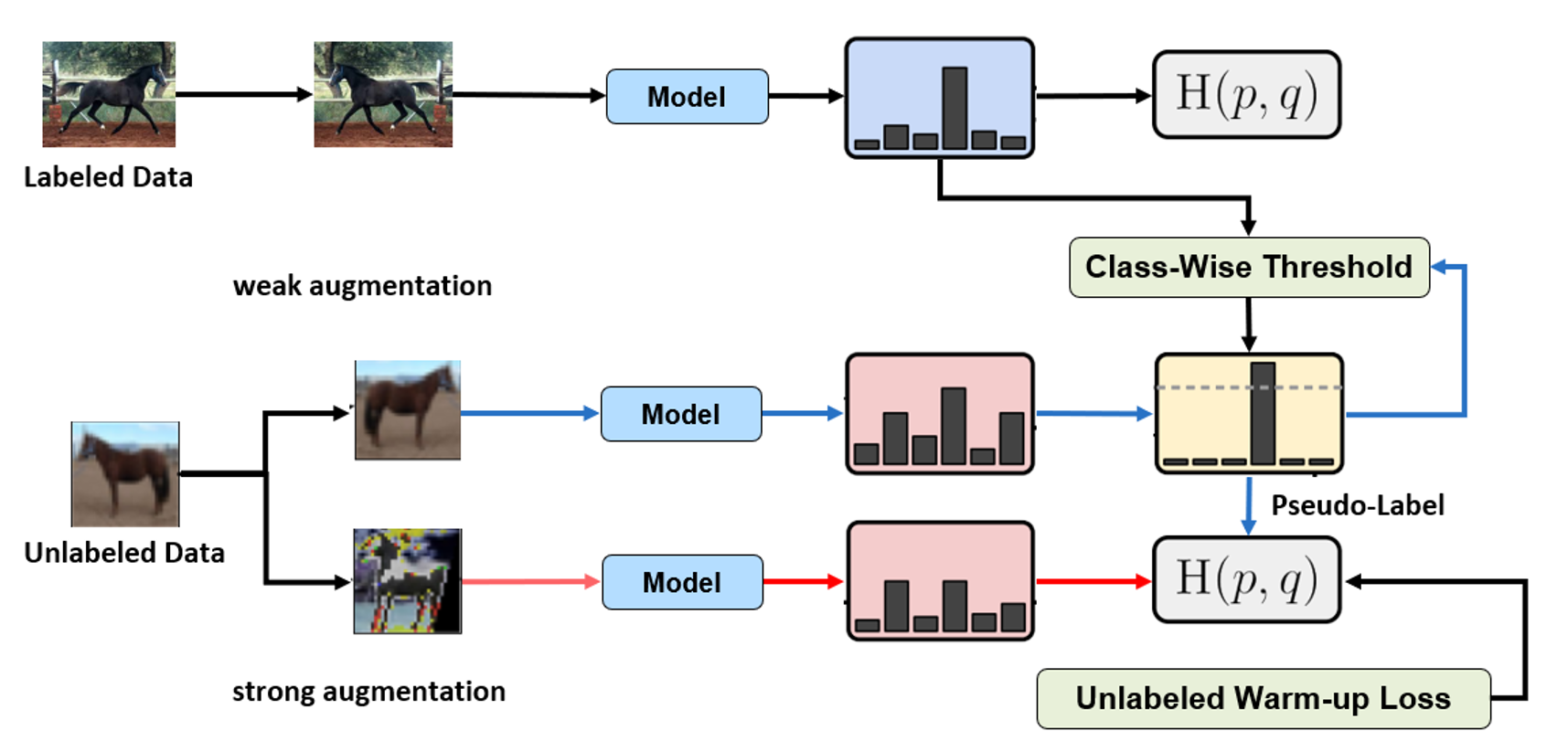
We use FixMatch as a core algorithm for Semi-SL task solving. It is a specific implementation of Semi-SL that has been shown to be effective in various applications. FixMatch introduces pseudo-labeling, which is the process of generating labels for the unlabeled data and treating them as if they were labeled data. Pseudo-labeling is based on the idea that the model’s prediction for the unlabeled data is likely to be correct, which can improve the model’s accuracy and reduce the need for labeled data.
In Semi-SL, the pseudo-labeling process is combined with a consistency loss that ensures that the predictions of the model are consistent across augmented versions of the same data. This helps to reduce the impact of noisy or incorrect labels that may arise from the pseudo-labeling process. Additionally, our algorithm uses a combination of strong data augmentations to further improve the accuracy of the model.
Overall, OpenVINO™ Training Extensions utilizes powerful techniques for improving the performance of Semi-SL algorithm with limited labeled data. They can be particularly useful in domains where labeled data is expensive or difficult to obtain, and can help to reduce the time and cost associated with collecting labeled data.
Pseudo-labeling (FixMatch): A specific implementation of Semi-SL that combines the use of pseudo-labeling with a consistency loss, strong data augmentations, and a specific optimizer called Sharpness-Aware Minimization (SAM) to improve the performance of the model.Adaptable Threshold: A novel addition to our solution that calculates a class-wise threshold for pseudo-labeling, which can solve the issue of imbalanced data and produce high-quality pseudo-labels that improve the overall score.Unlabeled Warm-Up Loss: A technique for preventing the initial unstable learning of pseudo-labeling by increasing the coefficient of the unlabeled loss from 0 to 1.Additional techniques: Other than that, we use several solutions that apply to supervised learning (Augmentations, Early-Stopping, etc.)
Training time depends on the number of images and can be up to several times longer than conventional supervised learning.
The recipe that provides Semi-SL can be found below.
(otx) ...$ otx find --task MULTI_CLASS_CLS --pattern semisl
You can select the model configuration and run Semi-SL training with the command below.
(otx) ...$ otx train \
            --config {semi_sl_config_path} \
            --data_root {path_to_labeled_data} \
            --data.unlabeled_subset.data_root {path_to_unlabeled_data}
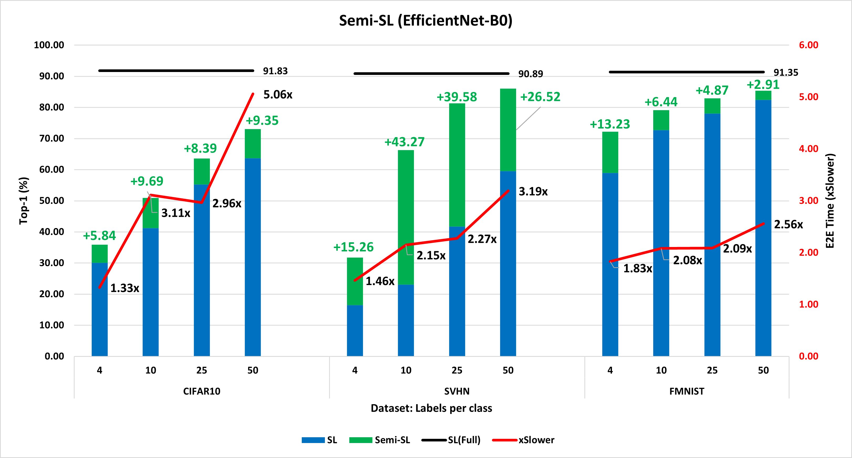
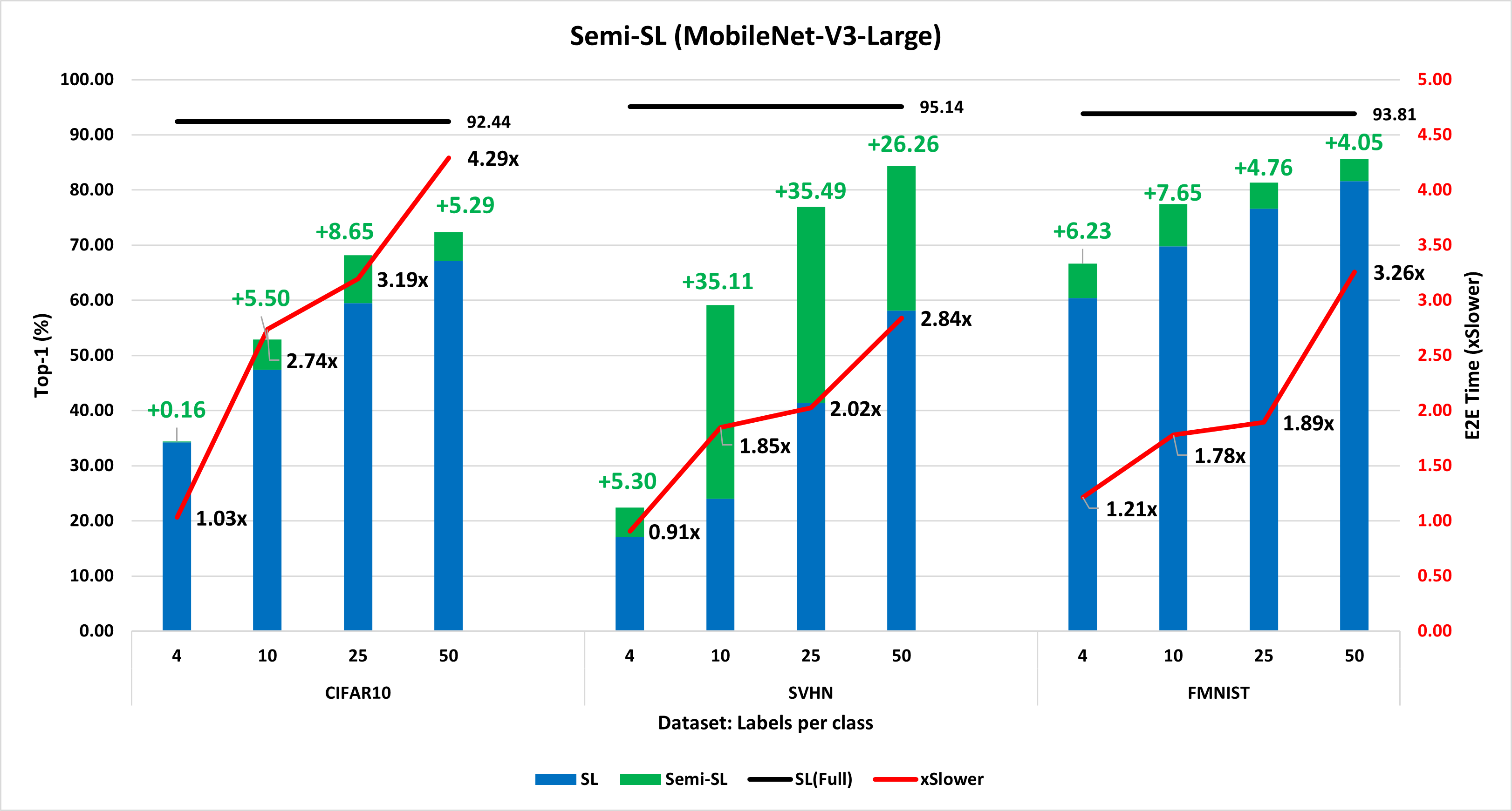
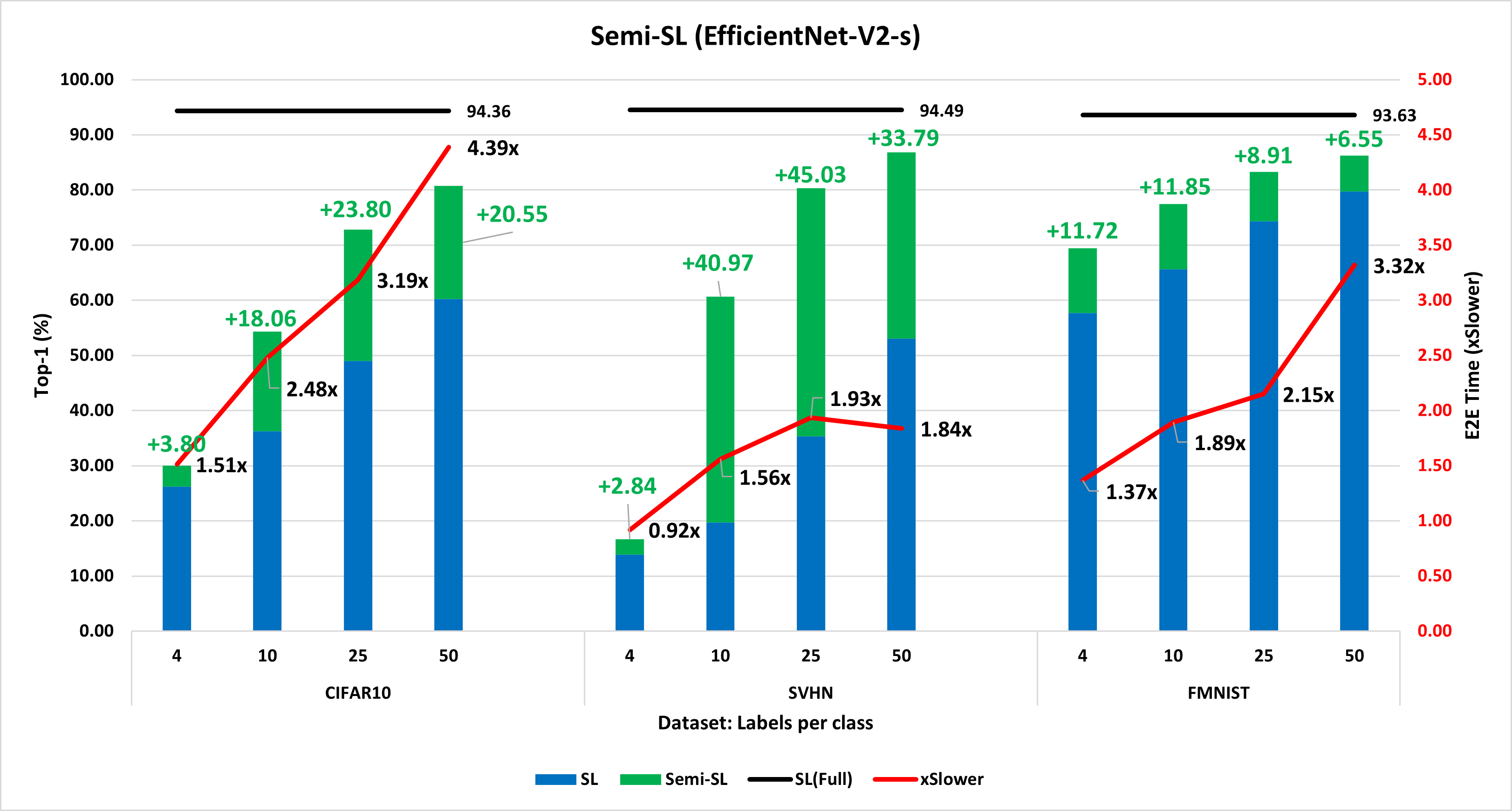
Below are the results of comparing supervised learning and semi-supervised learning for each label per class on three datasets, three models.
Model |
CIFAR10 |
SVHN |
FMNIST |
||||||||||
EfficientNet-B0 |
Labels per class |
4 |
10 |
25 |
50 |
4 |
10 |
25 |
50 |
4 |
10 |
25 |
50 |
SL |
top-1 (%) |
30.06 |
41.21 |
55.21 |
63.69 |
16.47 |
23.04 |
41.74 |
59.52 |
58.97 |
72.71 |
78.03 |
82.45 |
E2E time (s) |
121 |
95 |
141 |
143 |
287 |
233 |
241 |
228 |
107 |
135 |
162 |
154 |
|
Semi-SL |
top-1 (%) |
35.9 |
50.9 |
63.6 |
73.04 |
27.13 |
65.08 |
80.66 |
85.4 |
72.2 |
79.16 |
82.9 |
85.36 |
E2E time (s) |
160 |
295 |
417 |
722 |
419 |
500 |
549 |
728 |
196 |
281 |
339 |
395 |
Model |
CIFAR10 |
SVHN |
FMNIST |
||||||||||
MobileNet-V3-Large |
Labels per class |
4 |
10 |
25 |
50 |
4 |
10 |
25 |
50 |
4 |
10 |
25 |
50 |
SL |
top-1 (%) |
34.21 |
47.37 |
59.5 |
67.13 |
17.08 |
24.01 |
41.42 |
58.14 |
60.41 |
69.8 |
76.61 |
81.57 |
E2E time (s) |
109 |
127 |
153 |
159 |
333 |
277 |
254 |
287 |
141 |
135 |
126 |
136 |
|
Semi-SL |
top-1 (%) |
34.37 |
52.87 |
68.15 |
72.42 |
22.38 |
59.11 |
76.91 |
84.4 |
66.65 |
77.45 |
81.38 |
85.63 |
E2E time (s) |
112 |
348 |
489 |
684 |
302 |
512 |
515 |
815 |
172 |
240 |
238 |
442 |
Model |
CIFAR10 |
SVHN |
FMNIST |
||||||||||
EfficientNet-V2-S |
Labels per class |
4 |
10 |
25 |
50 |
4 |
10 |
25 |
50 |
4 |
10 |
25 |
50 |
SL |
top-1 (%) |
26.19 |
36.23 |
49.01 |
60.22 |
13.85 |
19.71 |
35.5 |
53.05 |
57.7 |
65.61 |
74.34 |
79.71 |
E2E time (s) |
110 |
128 |
149 |
165 |
322 |
308 |
325 |
407 |
149 |
113 |
142 |
163 |
|
Semi-SL |
top-1 (%) |
29.99 |
54.29 |
72.8 |
80.77 |
16.68 |
60.68 |
80.34 |
86.84 |
69.41 |
77.46 |
83.25 |
86.26 |
E2E time (s) |
166 |
318 |
475 |
726 |
297 |
481 |
629 |
748 |
204 |
215 |
305 |
542 |
Overall, you can expect to see an increase in metric scores, albeit slower than Supervised learning.