Semantic Segmentation#

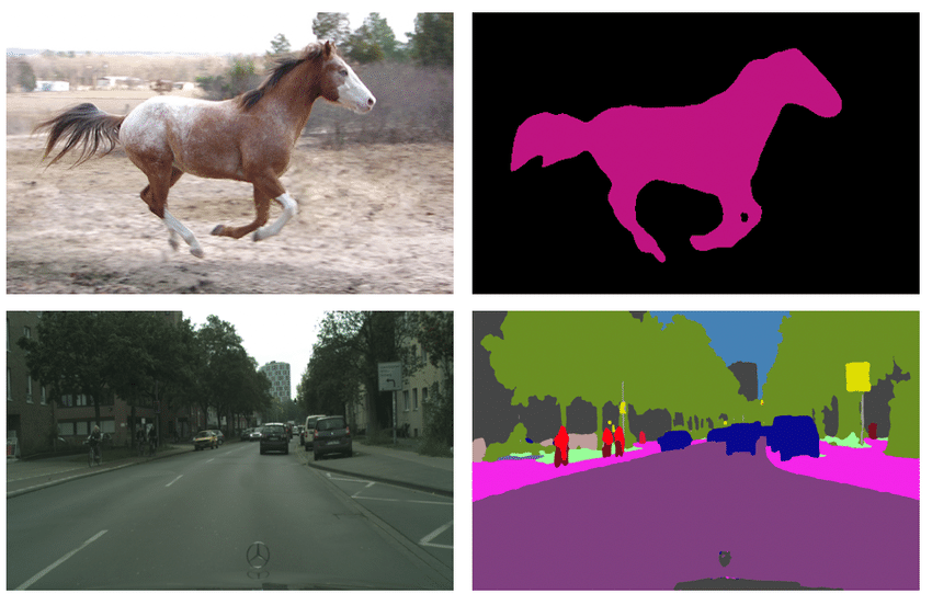
Semantic segmentation is a computer vision task in which an algorithm assigns a label or class to each pixel in an image. For example, semantic segmentation can be used to identify the boundaries of different objects in an image, such as cars, buildings, and trees. The output of semantic segmentation is typically an image where each pixel is colored with a different color or label depending on its class.

image uploaded from this `source <https://arxiv.org/abs/1912.03183>`_

We solve this task by utilizing FCN Head with implementation from MMSegmentation on the multi-level image features obtained by the feature extractor backbone (Lite-HRNet). For the supervised training we use the following algorithms components:

  • Augmentations: Besides basic augmentations like random flip, random rotate and random crop, we use mixing images technique with different photometric distortions.

  • Optimizer: We use Adam optimizer with weight decay set to zero and gradient clipping with maximum quadratic norm equals to 40.

  • Learning rate schedule: For scheduling training process we use ReduceLROnPlateau with linear learning rate warmup for 100 iterations. This method monitors a target metric (in our case we use metric on the validation set) and if no improvement is seen for a patience number of epochs, the learning rate is reduced.

  • Loss function: We use standard Cross Entropy Loss to train a model.

  • Additional training techniques
    • Early stopping: To add adaptability to the training pipeline and prevent overfitting. You can use early stopping like the below command.

      $ otx train {TEMPLATE} ... \
                  params \
                  --learning_parameters.enable_early_stopping=True
      

Dataset Format#

For the dataset handling inside OpenVINO™ Training Extensions, we use Dataset Management Framework (Datumaro).

At this end we support Common Semantic Segmentation data format. If you organized supported dataset format, starting training will be very simple. We just need to pass a path to the root folder and desired model template to start training:

$ otx train  <model_template> --train-data-roots <path_to_data_root> \
                                        --val-data-roots <path_to_data_root>

Note

Due to some internal limitations, the dataset should always consist of a “background” label. If your dataset doesn’t have a background label, rename the first label to “background” in the meta.json file.

Note

Currently, metrics with models trained with our OTX dataset adapter can differ from popular benchmarks. To avoid this and train the model on exactly the same segmentation masks as intended by the authors, please, set the parameter use_otx_adapter to False.

Models#

We support the following ready-to-use model templates:

Template ID

Name

Complexity (GFLOPs)

Model size (MB)

Custom_Semantic_Segmentation_Lite-HRNet-s-mod2_OCR

Lite-HRNet-s-mod2

1.44

3.2

Custom_Semantic_Segmentation_Lite-HRNet-18-mod2_OCR

Lite-HRNet-18-mod2

2.82

4.3

Custom_Semantic_Segmentation_Lite-HRNet-x-mod3_OCR

Lite-HRNet-x-mod3

9.20

5.7

All of these models are members of the same Lite-HRNet backbones family. They differ in the trade-off between accuracy and inference/training speed. Lite-HRNet-x-mod3 is the template with heavy-size architecture for accurate predictions but it requires long training. Whereas the Lite-HRNet-s-mod2 is the lightweight architecture for fast inference and training. It is the best choice for the scenario of a limited amount of data. The Lite-HRNet-18-mod2 model is the middle-sized architecture for the balance between fast inference and training time.

Besides this, we added new templates in experimental phase. For now, they support only supervised incremental training type. To run training with new templates we should use direct path to template_experimental.yaml.

Template ID

Name

Complexity (GFLOPs)

Model size (MB)

Custom_Semantic_Segmentation_SegNext_T

SegNext-t

6.07

4.23

Custom_Semantic_Segmentation_SegNext_S

SegNext-s

15.35

13.9

Custom_Semantic_Segmentation_SegNext_B

SegNext-b

32.08

27.56

New templates use SegNext model which can achieve superior perfomance while preserving fast inference and fast training.

In the table below the Dice score on some academic datasets using our supervised pipeline is presented. We use 512x512 image crop resolution, for other hyperparameters, please, refer to the related template. We trained each model with single Nvidia GeForce RTX3090.

Model name

DIS5K

Cityscapes

Pascal-VOC 2012

KITTI full

Mean

Lite-HRNet-s-mod2

79.95

62.38

58.26

36.06

59.16

Lite-HRNet-18-mod2

81.12

65.04

63.48

39.14

62.20

Lite-HRNet-x-mod3

79.98

59.97

61.9

41.55

60.85

SegNext-t

85.05

70.67

80.73

51.25

68.99

SegNext-s

85.62

70.91

82.31

52.94

69.82

SegNext-b

87.92

76.94

85.01

55.49

73.45

Note

Please, refer to our dedicated tutorial for more information on how to train, validate and optimize the semantic segmentation model.

Semi-supervised Learning#

We employ the Mean Teacher framework to tackle the problem of Semi-supervised learning in semantic segmentation. This framework leverages two models during training: a “student” model, which serves as the primary model being trained, and a “teacher” model, which acts as a guiding reference for the student model.

During training, the student model is updated using both ground truth annotations (for labeled data) and pseudo-labels (for unlabeled data). These pseudo-labels are generated by the teacher model’s predictions. Notably, the teacher model’s parameters are updated based on the moving average of the student model’s parameters. This means that backward loss propagation is not utilized for updating the teacher model. Once training is complete, only the student model is used for making predictions in the semantic segmentation task.

The Mean Teacher framework utilizes the same core algorithm components as the supervised pipeline for semantic segmentation. However, there are some key differences in the augmentation pipelines used for labeled and unlabeled data. Basic augmentations such as random flip, random rotate, and random crop are employed for the teacher model’s input. On the other hand, stronger augmentations like color distortion, RGB to gray conversion, and CutOut are applied to the student model. This discrepancy helps improve generalization and prevents unnecessary overfitting on the pseudo-labels generated by the teacher model. Additionally, pixels with high entropy, which are deemed unreliable by the teacher model, are filtered out using a schedule that depends on the training iterations.

For new experimental templates (SegNext family) we also adopted the prototype view approach which is based on two research works: Rethinking Semantic Segmentation: A Prototype View by Tianfei Zhou et al. and Semi-supervised Semantic Segmentation with Prototype-based Consistency Regularization by Hai-Ming Xu et al. We implemented a prototype network and incorporated it into the base Mean Teacher framework. We set weights for losses empirically after extensive experiments on the datasets presented below.

The table below presents the Dice score achieved by our templates on various datasets. We provide these scores for comparison purposes, alongside the supervised baseline trained solely on labeled data. We use 512x512 image resolution, for other hyperparameters, please, refer to the related templates. When training the new SegNext templates, we disabled early stopping and trained them for the full number of epochs. We trained each model with a single Nvidia GeForce RTX3090. For Cityscapes and Pascal-VOC we use splits with 1/16 ratio of labeled to unlabeled data like here. For other datasets, we prepared different numbers of classes and used the random split of the train data to obtain labeled and unlabeled sets.

  • VOC_12: 2 classes (person, car) were selected, 12 labeled images, 500 unlabeled and 150 images for validation

  • KITTI_54: 3 classes (vehicle, human, construction) were selected, 54 labeled images, 200 unlabeled and 50 images for validation

  • City_4: 4 classes (fence, vegetation, car, truck) were selected, 53 labeled images, 800 unlabeled and 500 images for validation

  • DIS5K 1/4: 1 class (objects), 242 labeled images, 728 unlabeled and 281 images for validation

Other classes for these datasets are marked as background labels.

Model name

Cityscapes

Pascal-VOC

DIS5K

VOC_12

KITTI_54

City_4

Mean mDice

Lite-HRNet-s-mod2

40.80

43.05

81.00

60.12

61.83

66.72

58.92

Lite-HRNet-18-mod2

42.71

44.42

81.18

63.24

61.4

67.97

60.15

Lite-HRNet-x-mod3

49.20

43.87

81.48

63.96

59.76

68.08

61.06

Lite-HRNet-s-mod2-SSL

45.05

44.01

81.46

64.78

61.90

67.03

60.71

Lite-HRNet-18-mod2-SSL

48.65

46.24

81.52

65.64

65.25

68.11

62.57

Lite-HRNet-x-mod3-SSL

50.00

46.10

82.00

66.10

66.50

68.41

63.19

SegNext-t

55.93

73.82

86.87

68.00

62.35

68.30

69.21

SegNext-s

63.75

77.24

87.88

76.30

66.45

69.34

73.49

SegNext-b

66.39

80.52

89.62

78.65

70.45

69.68

75.89

SegNext-t-SSL

60.2

77.44

87.60

70.72

67.43

69.21

72.10

SegNext-s-SSL

68.06

80.55

88.72

77.00

68.70

69.73

75.46

SegNext-b-SSL

71.80

82.43

90.32

80.68

73.73

70.02

78.16

Self-supervised Learning#

Self-supervised learning can be one of the solutions if the user has a small data set, but label information is not yet available. General self-supervised Learning in academia is commonly used to obtain well-pretrained weights from a source dataset without label information. However, in real-world industries, it is difficult to apply because of small datasets, limited resources, or training in minutes.

For these cases, OpenVINO™ Training Extensions provides improved self-supervised learning recipes that can be applied to the above harsh environments. OpenVINO™ Training Extensions allows to perform a pre-training phase on any images to further use obtained weights on the target dataset. We adapted DetCon as our self-supervised method. It takes some time to use these self-supervised learning recipes, but you can expect improved performance, especially in small-data regimes.

The below table shows how much performance (mDice) self-supervised methods improved compared with baseline performance on the subsets of Pascal VOC 2012 with three classes (person, car, bicycle). To get the below performance, we had two steps:

  • Train the models using only images containing at less one class of the three classes without label information to get pretrained weights for a few epochs.

  • Fine-tune the models with pretrained weights using subset datasets and get performance.

We additionally obtained baseline performance from supervised learning using subset datasets for comparison. Each subset dataset has 8, 16, and 24 images, respectively.

Model name

#8

#16

#24

SL

Self-SL

SL

Self-SL

SL

Self-SL

Lite-HRNet-s-mod2

48.30

53.55

57.08

58.96

62.40

63.46

Lite-HRNet-18-mod2

53.47

49.20

56.69

58.72

62.81

63.63

Lite-HRNet-x-mod3

50.23

50.93

60.09

61.61

62.66

64.87

Unlike other tasks, two things are considered to use self-supervised learning:

  • --train-data-roots must be set to a directory only containing images, not ground truths. DetCon uses pseudo masks created in detcon_mask directory for training. If they are not created yet, they will be created first.

  • --val-data-roots is not needed.

To enable self-supervised training, the command below can be executed:

$ otx train Lite-HRNet-18-mod2 \
            --train-data-roots path/to/images \

After self-supervised training, pretrained weights can be use for supervised (incremental) learning like the below command:

$ otx train Lite-HRNet-18-mod2 \
            --train-data-roots path/to/train/subset \
            --val-data-roots path/to/validation/subset \
            --load-weights={PATH/PRETRAINED/WEIGHTS}

Note

SL stands for Supervised Learning.

Supervised Contrastive Learning#

To enhance the performance of the algorithm in case when we have a small number of data, Supervised Contrastive Learning (SupCon) can be used.

More specifically, we train a model with two heads: segmentation head with Cross Entropy Loss and contrastive head with DetCon loss. As of using this advanced approach, we can expect improved performance and reduced training time rather than supervised learning. The below table shows how much performance (mDice) SupCon improved compared with baseline performance on the subsets of Pascal VOC 2012 with three classes (person, car, bicycle). Each subset dataset has 8, 16, and 24 images, respectively.

Model name

#8

#16

#24 |

SL

SupCon

TR

SL

SupCon

TR

SL | SupCon

TR

Lite-HRNet-s-mod2

52.30

54.24

0.83x

59.58

61.44

0.93x

62.86

64.30

1.03x

Lite-HRNet-18-mod2

53.00

56.16

0.71x

61.44

60.08

0.91x

64.26

64.82

0.91x

Lite-HRNet-x-mod3

53.71

58.67

0.83x

58.43

61.52

0.73x

64.72

65.83

0.73x

The SupCon training can be launched by adding additional option to template parameters like the below. It can be launched only with supervised (incremental) training type.

$ otx train Lite-HRNet-18-mod2 \
            --train-data-roots path/to/train/subset \
            --val-data-roots path/to/validation/subset \
            params \
            --learning_parameters.enable_supcon=True

Note

SL : Supervised Learning / TR : Training Time Ratio of SupCon compared with supervised learning